Tutorial 06: Calculating the density and heat capacity of an \(O_2\) plasma.

The most common use of minplascalc is the calculation of thermophysical properties of plasmas in LTE. In this example we’ll look at the thermodynamic properties \(\rho\) and \(c_p\).

The relatively simple case of a pure oxygen plasma is useful for demonstration and validation purposes. As in Tutorial 05: Calculating equilibrium compositions for an O_2 plasma., a Mixture object must be created by the user to specify the plasma species present and the relative proportions of elements. We’ll use a system identical to the previous example.

Import the required libraries.

We start by importing the modules we need:

• matplotlib for drawing graphs,

• numpy for array functions,

• and of course minplascalc.

import matplotlib.pyplot as plt
import numpy as np

import minplascalc as mpc

Create mixture object for the species we’re interested in.

Next, we create a minplascalc LTE mixture object. Here we use a helper function in minplascalc which creates the object directly from a list of the species names.

oxygen_mixture = mpc.mixture.lte_from_names(
    ["O2", "O2+", "O", "O-", "O+", "O++"], [1, 0, 0, 0, 0, 0], 1000, 101325
)

Set a range of temperatures to calculate the equilibrium compositions at.

Next, set a range of temperatures to calculate the equilibrium compositions at - in this case we’re going from 1000 to 25000 K in 100 K steps. Also initialise a list to store the property values at each temperature.

temperatures = np.linspace(1000, 25000, 100)
density = []
cp = []
h = []

Perform the composition calculations.

Now we can perform the property calculations. We loop over all the temperatures setting the mixture object’s temperature attribute to the appropriate value, and calculating the plasma density by calling the LTE object’s calculate_density() and calculate_heat_capacity() functions. Internally, these make calls to calculate_composition() to obtain the composition of the plasma before the calculation of the properties.

Note that execution of this calculation is fairly compute intensive and the following code snippet may take several seconds to complete.

for T in temperatures:
    oxygen_mixture.T = T
    density.append(oxygen_mixture.calculate_density())
    cp.append(oxygen_mixture.calculate_heat_capacity())
    h.append(oxygen_mixture.calculate_enthalpy())

Plot the results.

Now we can visualise the properties by plotting them against temperature, to see how they vary.

fig, axs = plt.subplots(1, 3, figsize=(10, 4))

ax = axs[0]
ax.set_title(r"$\mathregular{O_2}$ plasma density at 1 atm")
ax.set_xlabel("T [K]")
ax.set_ylabel("$\\mathregular{\\rho [kg/m^3]}$")
ax.semilogy(temperatures, density, "k", label="minplascalc")
ax.legend()

ax = axs[1]
ax.set_title(r"$\mathregular{O_2}$ plasma heat capacity at 1 atm")
ax.set_xlabel("T [K]")
ax.set_ylabel(r"$\mathregular{C_P [J/(kg.K)]}$")
ax.plot(temperatures, cp, "k", label="minplascalc")
ax.legend()

ax = axs[2]
ax.set_title(r"$\mathregular{O_2}$ plasma enthalpy at 1 atm")
ax.set_xlabel("T [K]")
ax.set_ylabel(r"$\mathregular{H [J/kg]}$")
ax.plot(temperatures, h, "k", label="minplascalc")
ax.legend()

plt.tight_layout()

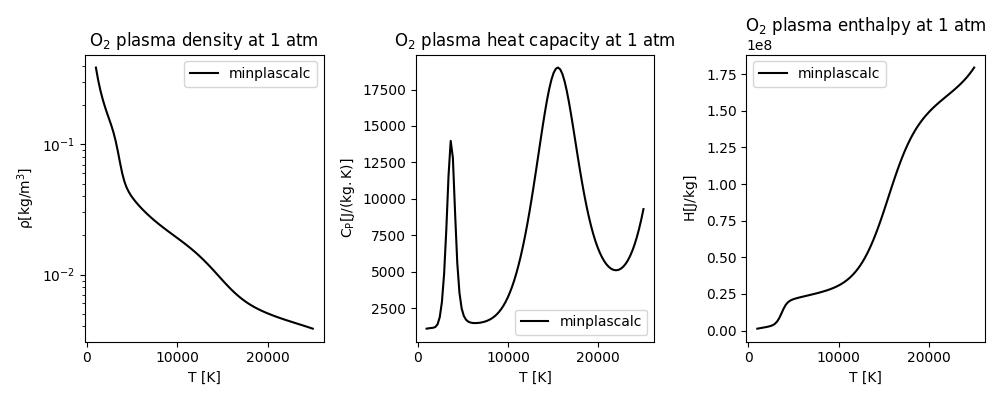
Conclusion

The results obtained using minplascalc are comparable to other data for oxygen plasmas in literature, for example [Boulos2023]. In particular the position and size of the peaks in \(C_p\), which are caused by the highly nonlinear dissociation and first ionisation reactions of \(O_2\) and \(O\) respectively, are accurately captured.