Tutorial 09: Calculating the density and heat capacity of an SiO-CO plasma.

The most common use of minplascalc is expected to be the calculation of thermophysical properties of plasmas in LTE as a function of elemental composition, temperature, and pressure. For the more complex SiO-CO plasma, mixtures must be created as described in Tutorial 08: Calculating equilibrium compositions of an SiO-CO plasma. to specify the plasma species present and the relative proportions of elements.

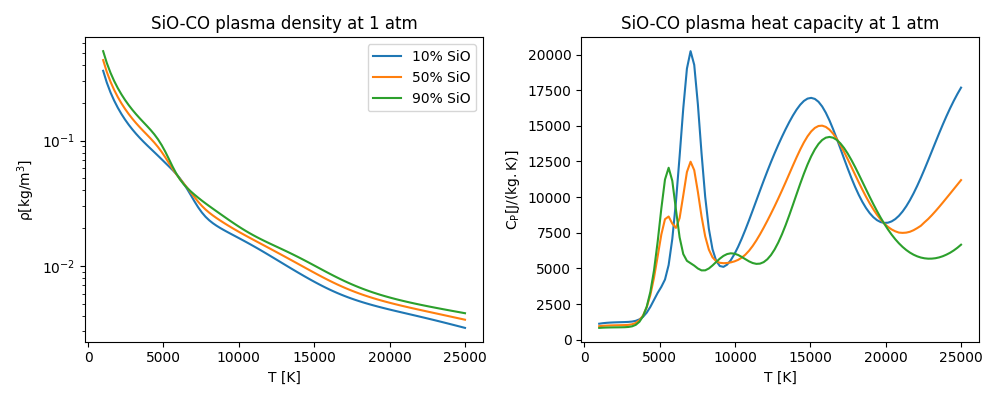
For this tutorial we’ll look at three different SiO-CO mixtures ranging from 10% SiO to 90% SiO by mole to show how the properties are affected by different mixture ratios.

Import the required libraries.

We start by importing the modules we need:

• matplotlib for drawing graphs,

• numpy for array functions,

• and of course minplascalc.

import matplotlib.pyplot as plt
import numpy as np

import minplascalc as mpc

Create mixture object for the species we’re interested in.

Next, we create some minplascalc LTE mixture objects as before.

species = [
    "O2",
    "O2+",
    "O",
    "O+",
    "O++",
    "CO",
    "CO+",
    "C",
    "C+",
    "C++",
    "SiO",
    "SiO+",
    "Si",
    "Si+",
    "Si++",
]
x0s = [
    [0, 0, 0, 0, 0, 1 - sio, 0, 0, 0, 0, sio, 0, 0, 0, 0]
    for sio in [0.1, 0.5, 0.9]
]
sico_mixtures = [
    mpc.mixture.lte_from_names(species, x0, 1000, 101325) for x0 in x0s
]

Set a range of temperatures to calculate the equilibrium compositions at.

Next, set a range of temperatures to calculate the equilibrium compositions at - in this case we’re going from 1000 to 25000 K in 100 K steps. Also initialise a list to store the property values for the various mixture at each temperature.

temperatures = np.linspace(1000, 25000, 100)
densities: list[list[float]] = [[], [], []]
heat_capacities: list[list[float]] = [[], [], []]

Perform the composition calculations.

Now we can perform the property calculations. We loop over all the temperatures setting the mixture object’s temperature attribute to the appropriate value, and calculating the plasma density by calling the LTE object’s calculate_density() and calculate_heat_capacity() functions. Internally, these make calls to calculate_composition() to obtain the composition of the plasma before the calculation of the properties.

Note that execution of this calculation is fairly compute intensive and the following code snippet may take a couple minutes or more to complete.

for i, sico_mixture in enumerate(sico_mixtures):
    for T in temperatures:
        sico_mixture.T = T
        densities[i].append(sico_mixture.calculate_density())
        heat_capacities[i].append(sico_mixture.calculate_heat_capacity())

Plot the results.

Now we can visualise the properties by plotting them against temperature, to see how they vary.

fig, axs = plt.subplots(1, 2, figsize=(10, 4))

labels = ["10% SiO", "50% SiO", "90% SiO"]

ax = axs[0]
ax.set_title("SiO-CO plasma density at 1 atm")
ax.set_xlabel("T [K]")
ax.set_ylabel("$\\mathregular{\\rho [kg/m^3]}$")
for density, label in zip(densities, labels):
    ax.semilogy(temperatures, density, label=label)
ax.legend()

ax = axs[1]
ax.set_title("SiO-CO plasma heat capacity at 1 atm")
ax.set_xlabel("T [K]")
ax.set_ylabel(r"$\mathregular{C_P [J/(kg.K)]}$")
for heat_capacity, label in zip(heat_capacities, labels):
    ax.plot(temperatures, heat_capacity, label=label)

plt.tight_layout()

Conclusion

The impact of changing the elemental composition of the plasma is quite marked, particularly in the case of the heat capacity - the multiple overlapping peaks representing dissociation and ionisation of the various species move around considerably depending on whether the plasma is formed from mostly SiO, or mostly CO. The general trend is toward slightly lower values of \(C_p\) and slightly higher values of \(\rho\) for SiO-rich plasmas, but it does depend which temperature regime is being considered.